The wildcard character and SUMPRODUCT are like oil and water, they just don’t gel well together. The beauty of SUMPRODUCT is somewhat tarnished with its inability to play nicely with the Wildcard * character. It works well with SUMIFS and other Excel Functions but not with SUMPRODUCT. The focus of this article will be to demonstrate how to work around this constraint using a number of examples.
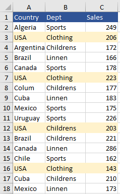
Take the following data set for example, we have countries in Column A and Departments in Column B.
Ideally we Sum by Country by the Department. If we want ALL departments the natural choice is SUMIFS. Where the following gets the job done:
=SUMIFS(C2:C19,A2:A19,E2,B2:B19,"*")
The wildcard character is your friend and works beautifully with SUMIFS. The SUMPRODUCT formula is a different beast and will need formulas such as LEN to take the place of the wildcard.
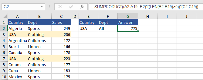
I recently stumbled across an idea, what if we tested the length of the characters in a given range, with the LEN formula, then summed all of the instances where the length of the cells were greater than 1 character long. This would be the same as the wildcard character. You could then string a range of criteria matches after this point embedded in the SUMPRODUCT formula.
=SUMPRODUCT((A2:A19=E2)*((LEN(B2:B19)>0))*(C2:C19))
It works nicely and summarises the data well.
The SUMPRODUCT formula above cuts through the data set and summarises the data well. However, in the above example where there is only one column to sum then the SUMIFS is the best option. It is a lighter touch and the formula is simpler.
Whenever faced with the problem of summing a single column with criteria or the entire column (the sum of the parts) the SUMIFS and the INDEX and MATCH in a nested formula has helped by solving the problem in the past or the use of a helper column which sums year to date and then use as SUMIFS formula. This is a tad complex though. Also if you have 10,000 lines of data you will need an additional 10,000 formula to get YTD just to use a single SUMIFS formula to calculate your summary.
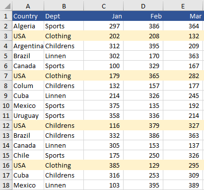
Enter the SUMPRODUCT formula in conjunction with the LEN formula (this example makes the assumption of a full dataset with information being filled for both country and department - no blanks).
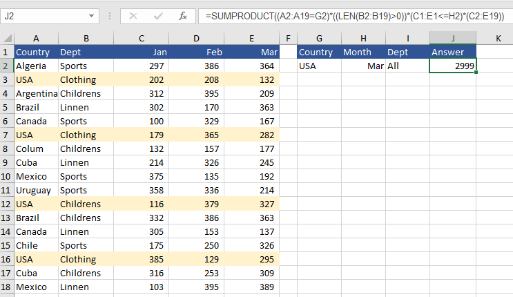
To generate a summary on data based in the country of USA and all year to date data prior to March we need USA as criteria, our LEN formula for all Departments and less than or equal to <= March as criteria. This should produce a result.
=SUMPRODUCT((A2:A19=G2)*((LEN(B2:B19)>0))*(C1:E1<=H2)*(C2:E19))
The above works well on all criteria. It sums USA, ALL departments and every transaction greater than or equal to March for a seamless YTD calculation.
The following file should help crystallise the concept for you


