In Excel you don't need to be bound by conditional formatting to colour a cell in the format you wish. For example, you may wish to colour the format of a cell in the Format Cell dialog, in the process you may well just be making your spreadsheet run a little quicker. Using conditional formatting to do the same task can slow the smooth operation of a file on occasion. Conditional formatting is volatile by nature meaning it needs more horse power to run. Setting the format "in cell" will use less resource and make your spreadsheet run faster. All good :)
The following YouTube video takes you through a few examples.
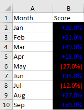
The following formula with example says if the cells value is greater than zero then the text will appear as green(with a plus + sign before hand), otherwise it will appear as red in brackets.
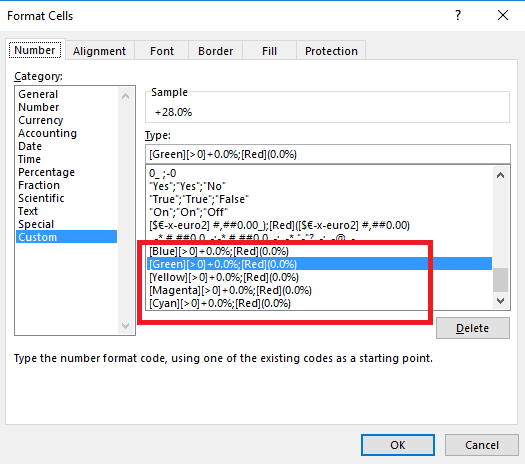
[Green][>0]+0.0%;[Red](0.0%)
You may wish to add variations to this condition such as adding a plus sign and changing the colour - here in blue.
[Blue][>0]+0.0%;[Red](0.0%)
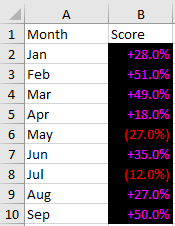
While here is yet another example in magenta.
[Magenta][>0]+0.0%;[Red](0.0%)
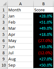
While the following uses Cyan.
[Cyan][>0]+0.0%;[Red](0.0%)
Create the Formatting
The set up occurs in the format cells section. Right click the cell - Format Cells.
Choose the Format Cells option from the list.
In the Type box paste any of the suggested formaula and then take your pick from the range of options we just created.
Or you could add a bit more pizzas to your format by adding a shape. The following is taken from the Aerial library.
See how the formatting is different for positive and negative values. The addition of a symbol is neat. To left align the symbol I used a * wildcard symbol. Incidentally to right align use the @ symbol. Here is the formula used in the above example.
[Green][>0]●* 0.0%;[Red]●* (0.0%)
The following is the Excel file to show the workings.


