This post is a follow up from the blog post earlier in the month on Filtering without a filter. It is an alternative to the autofilter method I have outlined extensively. The post focuses on filtering out more than one criteria and putting the results in a fresh sheet. To do so we use the evaluate method. This is relatively complex, however if we break down what needs to change we can significantly simplify the process.
What we will do is to test if there is No or Maybe in column 3 of our dataset. If so we want to move all of those cells to the next sheet called Res.
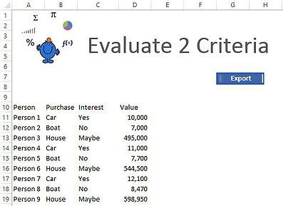
For starters our data set is simple and looks as follows:
The headers start in row 10 and the dataset is 4 columns in width. Firstly we test if there is data in column 3 which says the word yes. If not there is no need to run the procedure.
If Application.CountIf(Sheet1.Columns(3), "Yes") = 0 Then Exit Sub
Then we tell VBA where the dataset starts from (row 10).
With Sheet1.[a10].CurrentRegion
Now we set the variant (ar).
ar = Filter(.Parent.Evaluate("transpose(if((" & .Columns(Col).Address & _
"=""No"")+(" & .Columns(Col).Address & "=""Maybe""),row(1:" & _
.Rows.Count & "),char(Col)))"), Chr(2), 0)
The above is the complex part but knowing what to change is all important. The column we wish to evaluate is column 3. That column (which says Interest) has the Yes, No or Maybe in it. The following variable:
Dim Col As Integer
Col = 3
It has been included to help with this procedure. Put the column number you are evaluating in after col = ?
Where the question mark represents your column to evaluate.
The next part to change is how large you want the array and which columns you want to include in your output. In the folowing example 4 columns.
ar = Application.Index(.Value, Application.Transpose(ar), [{1,2,3,4}])
The above includes 4 columns in the array Ar. If you wanted for example columns 1 and 4 the code would look as follows:
ar = Application.Index(.Value, Application.Transpose(ar), [{1,4}])
If you did change that part you would need to change the size of the output array which is next.
Sheet2.[A2].Resize(UBound(ar, 1), 2).Value = ar
Where 2 is equal to columns (1 and 4). In the full version of this example we will include all 4 columns. The procedure is as follows:
Option Explicit
Sub FilterToNewLoc2Crit()
Dim ar As Variant
Dim Col As Integer
Col = 3
If Application.CountIf(Sheet1.Columns(3), "Yes") = 0 Then Exit Sub
With Sheet1.[a10].CurrentRegion
ar = Filter(.Parent.Evaluate("transpose(if((" & .Columns(Col).Address & _
"=""No"")+(" & .Columns(Col).Address & "=""Maybe""),row(1:" & _
.Rows.Count & "),char(2)))"), Chr(2), 0)
ar = Application.Index(.Value, Application.Transpose(ar), [{1,2,3,4}])
End With
Sheet2.[A2].Resize(UBound(ar, 1), 4).Value = ar
End Sub
You will notice the output of this Excel VBA macro goes to sheet2 (the sheet code name). I will attach a file to show a working version of this method. I still prefer the autofilter with VBA but this method I assume has real speed. You can read up on the autofilter method Autofilter.
The Excel file is below.


