Hiding Rows Quickly with VBA

Hiding rows with Excel VBA the simple way using a union range. Typically if you want to hide rows very fast with VBA the autofilter is the tool of choice, in a single line with one swift move thousands of rows can be hidden. It has always been my preferred method when dealing with multiple rows to hide. Recently I had a problem where I needed to use the filter on the same range for other purposes so had to asses each cell individually. If you know anything about VBA when the program has to loop over multiple cells it can lag, especially if it needs to perform an action after each iteration.

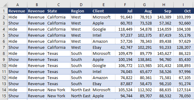
Enter the union array into the fray. This little diddy will do something similar to an autofilter where the data is hidden with single line. This drastically reduces the run time of the code as one action hides all of the rows in question. Imagine column A has the terms “Hide” and “Show”. The rows which say hide will be hidden and the rows that say show are visible. See example below.

The hide rows procedure needs to set a start point, an end point then a loop that runs from start to end. We set up two ranges Rng for the entire used column and r for the cell. Then it is a matter of looping through the 2 ranges and assigning the joined range to a 3rd range called JoinR. The JoinR range will be used in a Union Range which is a range that is made up of multiple often non consecutive ranges. We then use the union range to in essence hide all the rows that say hide. It is a fancy in memory way to perform the hide rows action once. This adds significant speed to the procedure.

The following is the set up for the procedure. Each line has a purpose.

Sheet1 is the Worksheet Code Name for the sheet named Hide. We always use the worksheet code name as if the tab name changes the code will not break. The lr is short for last row and the next line detects the last used row in the procedure. Finally the Rng variable is the first used row to the last used row. The following are the 3 set up lines.

Set sh = Sheet1 'BudInput tab
lr = sh.Range("A" & Rows.Count).End(xlUp).Row
Set Rng = sh.Range("A2:A" & lr)

The next thing to do is to create a looping construct. For every cell in the range we want to check to see if the cell says Hide. So starting from row 2 ending in the last used range. This is done by assigning a new variable to the cell being assessed. This variable is represented by r. The For loop is used with r being the single cell range and rng being the length of the range used in column A.

    For Each r In Rng

Next we check if r is equal to “Hide”

If r.Value = "Hide" Then

Here is where things get interesting, we are introducing a variable for a union range called JoinR. We need to check if our variable JoinR has anything in it. If it is blank we have to assign it to r, if not then we want to grow the range JoinR by simply adding to it.

The following checks if JoinR is not blank

If Not JoinR Is Nothing Then

If not blank then it will Set JoinR’s range to equal itself plus the cell represented by r, thus growing the range JoinR incrementally every time a “Hide” cell is encountered. If JoinR is blank and the cell equals hide then JoinR is assigned its first range as follows.

Set JoinR = r 'Trap the first instance of Hide

Where JoinR is equal to r. Now JoinR has a range verifiable attached to it and the line above that checks for a non blank range will kick in and continually add to the union range JoinR.

Finally after the looking and If statements are complete, the procedure hides the cells in the Uniion range JoinR once and the procedure ends. By hiding the rows one time the procedure saves a significant amount of time as opposed to hiding each row one by one. Performing actions inside conde continually is what causes VBA to lag and this procedure keeps that lag to a minimum and runs very quickly indeed. The following is the full procedure.

Sub HideRows()
Dim JoinR As Range
Dim Rng As Range
Dim sh As Worksheet
Dim r As Range
Dim lr As Long

Set sh = Sheet1 'Active sheet tab
lr = sh.Range("A" & Rows.Count).End(xlUp).Row 'Trap last row
Set Rng = sh.Range("A2:A" & lr) 'Trap start and end

    For Each r In Rng
        If r.Value = "Hide" Then
            If Not JoinR Is Nothing Then
                Set JoinR = Application.Union(JoinR, r) 'Trap every other instance
            Else
                Set JoinR = r   'Trap the first instance of Hide
            End If
        End If
    Next r
    
    JoinR.EntireRow.Hidden = True
End Sub

The final line JoinR.EntireRowHidden = True is the line where the Union Range cells are hidden. The action is performed once. I will attach a test file so you can see the procedure working on the example shown above. That should help to crystallise the concept of union ranges.

HideRows.XLSM