Recently I had an issue, there were two tables which were disconnected and I needed the first pivot table to be refreshed off the output of the second pivot table when these were using different data sources. I solved this problem with a little VBA and a worksheet change event. The following was the first list - notice the TOTAL at the bottom. This is important as I want to consolidate on my dashboard page with a slicer but I am using calculation tables and a single pivot tables to summarise the datasets. The file attached is a sample of a much larger dataset.
I have created a YouTube video outlining the procedure. The start file is as follows:
The following is the small list that the pivot table and slicer will be built on.
The above is the starting list with the ALL at the base. Creating a slicer off the raw data (not the above) looks as follows.
If all items are selected then that is the TOTAL - however if I want ta consolidation button for ALL I have to change it up a bit.
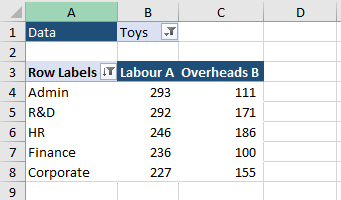
Now the database won’t have a field called ALL and this is important as I don’t want the user to click all the buttons (or unfilter everything) in order to show the TOTAL for all positions. Here is an example, it shows a pivot table summarised by ALL departments.
Notice the addition of ALL at the end of the slicer. This will be our consolidation and we will manipulate the pivot table when this disconnected slicer is clicked. The raw pivot table that will feed our summary is a top five by the labour column and it will look as follows:
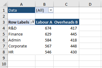
A summary by TOTAL is represented by the term ALL, so I want the pivot table to show the sum of the parts and I want the ability to summarise by ALL which is the TOTAL. The following is what ALL looks like:
There is a new disconnected list on the LIST Sheet and this will be used for the slicer to control the output sheet. This worksheet contains the pivot table the ultimate slicer is built upon.
Using VBA to Update the Pivot Table
As the two lists are from different datasets a little VBA code is needed. The code to change the pivot table is as follows.
Option Explicit

Sub ChangePiv()
  Dim PT As PivotTable
  Dim PF As PivotField
  Dim str As String

  Set PT = Sheet4.PivotTables("PivotTable1")
  Set PF = PT.PivotFields("List")
  str = Sheet2.[B1].Value

  PF.ClearAllFilters
  PF.CurrentPage = str

End Sub
There are a few things you will need to change above to match your data set. The first is the name of the worksheet code name
Sheet4
The next is the name of the name pivot table:
PivotTable1
The next is the name of your pivotfield:
“List”
An the final part is where the cell that you wish to control the pivot table is, be aware of the sheet it is on and the cell:
str = Sheet2.[B1].Value
You may want to do this from a data validation list or you could do it as I am presenting through a secondary slicer. Once these three things are changed you should be ready for the final part. This is creating the on cell change code that will run the macro every time your data validation list or slicer is clicked on.
The final bit of code need to go in the sheet that the slicer comes from - in my case it is the LIST tab worksheet code.
The ON Change Code
Option Explicit

Private Sub Worksheet_PivotTableChangeSync(ByVal Target As PivotTable)
    ChangePiv
End Sub
Inside the above code is the name of the macro that I want to run every time the pivot table changes and this will be through the slicer click.
The Final Product
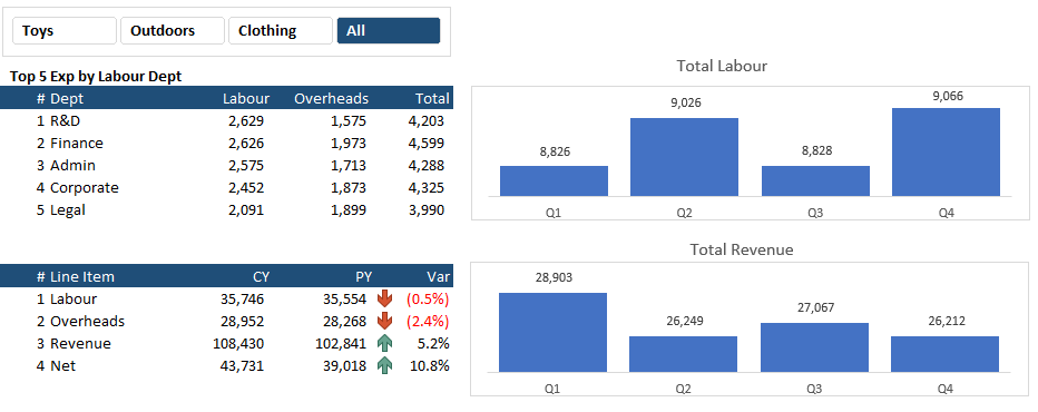
The following is what the model looks like once complete. I have enhanced it a little
It is a more intuitive method in my opinion of showing a total than by clicking all the buttons but others may feel differently. It is naturally a lot more work to create this method. Each to their own. The following Excel file should help you see the workings behind the above. You will need to understand the concept to apply it to your problem though. I will add a video in time to this article.


