Do Not Display Zero Values in a Chart
The following article shows how to display an Excel chart without zeros in the chart. The traditional method for excluding zero values is to use NA() with a condition see Remove Chart Series. This method is described in the article Here. The following is a slightly different method which uses named ranges for the graphs and an on Change event to sort the data as the Chart's underlying data changes. It works well if you are expecting zero values to muddy a well thought out Chart.
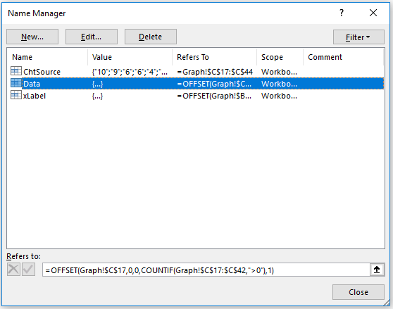
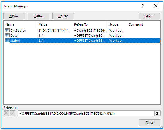
Add a value to any of the items under Stock which is zero and it will be added to the chart. Place a zero against any of the items with a value and it will be automatically removed from the Chart. The secret behind it is the two named ranges which feed the chart.
Data is the named range. The formula is as follows.
=OFFSET(Graph!$C$17,0,0,COUNTIF(Graph!$C$17:$C$42,">0"),1)
xLabel is the named range. The formula is as follows.
=OFFSET(Graph!$B$17,0,0,COUNTIF(Graph!$C$17:$C$42,">0"),1)
There is a VBA on Change Event which fires every time data between a range with ChtSource is changed. Note - a named range was created called ChtSource.
The length of the Range is not dynamic in the example above but has more cells than is required so further Fruits can be added to the list. Use any of the many dynamic range examples if you wish to extend the range. Also it is advisable you name cell C17. It will help make the code a little more error resistant.
In the above Example there has been a Range called Start Range put in the first cell which contains a number (C17).
The attached Excel file should help with learning.


