Update Chart from Dropdown

Updating a chart from a data validation dropdown is possible with the help of a dynamic range.  This method is similar to the Dynamic Updating Chart method with the advantage of adding a dropdown to update the chart.  

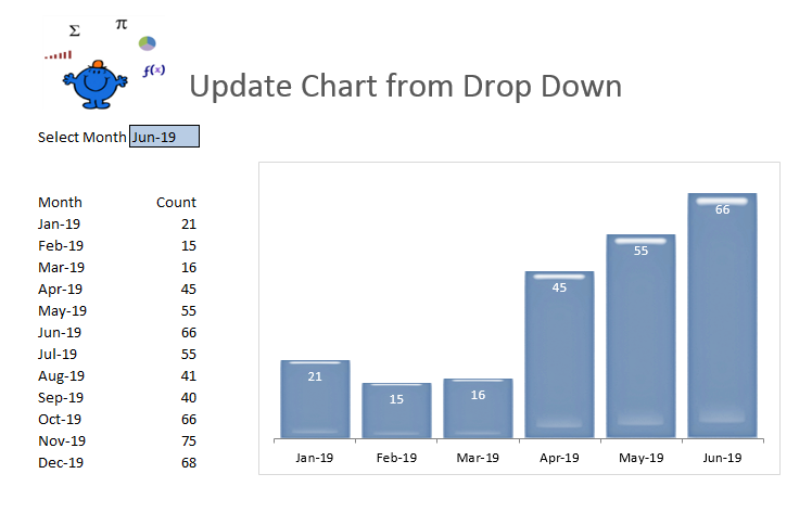
You can see from the above that the chart displays the first 7 months of the year.  This is in line with the cell in pink above.  As this cell changes so too does the chart.  For both of the dynamic ranges a named range is created.  The first dynamic range I have named Label and is as follows. To bring up the name manager Press Ctrl F3.

Choose New for a new named range and put the following formula in.

=OFFSET(Filter!$C$11,0,0,MATCH(Filter!$D$7,Filter!$C$11:$C$22,0),1)

This is the dynamic range for the labels (months) of the chart.  To generate the figures in the chart the following named range is used.

=OFFSET(Label,,1)

I have called this named range Figs.

To attach the labels to the chart right click on the chart and Select Data.

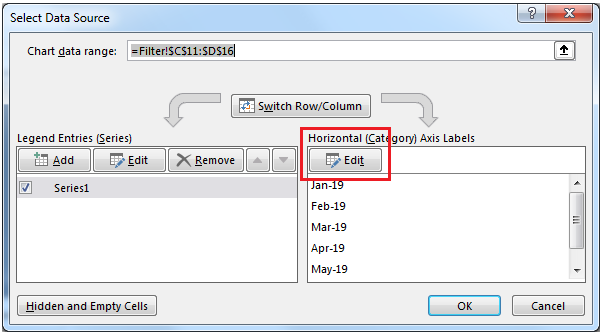
Click on the Edit button

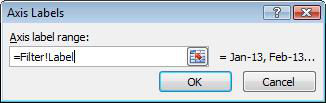
The sheet name is called Filter and after the exclamation mark ! put the word Label.  Follow the same procedure for the figures clicking on the Edit button for the Legend on the left in the table above.  The chart will now be dynamic based on the selection from the dropdown.  

The following Excel file show the workings from the above.  The procedure uses the formulas shown to change the chart based on the value in the drop down.  The procedure should be scalable with your Excel data.